44 add data labels to pivot chart
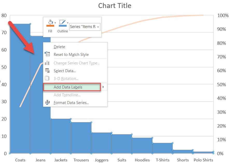
How to add data labels from different column in an Excel chart? Please do as follows: 1. Right click the data series in the chart, and select Add Data Labels > Add Data Labels from the context menu to add... 2. Right click the data series, and select Format Data Labels from the context menu. 3. In the Format Data Labels pane, under Label Options tab, check the ... Add data and format Pivot Chart using VBA Excel With pivotsheet.PivotTables("CHART_NAME") 'Insert Row Fields With .PivotFields("Country") .Orientation = xlRowField End With 'Insert Data Field With .PivotFields("Overdue") .Orientation = xlDataField .Function = xlCount .NumberFormat = "#,##0" .Name = "Number Overdue" End With End With
EOF

Add data labels to pivot chart
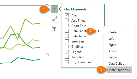
Change the format of data labels in a chart To get there, after adding your data labels, select the data label to format, and then click Chart Elements > Data Labels > More Options. To go to the appropriate area, click one of the four icons ( Fill & Line, Effects, Size & Properties ( Layout & Properties in Outlook or Word), or Label Options) shown here. Adding Data Labels to a Pivot Chart with VBA Macro ActiveSheet.ChartObjects ("Cluster Overview").Activate ActiveChart.FullSeriesCollection (1).DataLabels.Select For i = 1 To Range ("PivotTable1 [Project '#]").Count ActiveChart.FullSeriesCollection (1).Points (i).DataLabel.Select Selection.Formula = Range ("PivotTable1 [Project '#]").Cells (i, 1) Next i Any help you can give will be great. support.google.com › docs › answerAdd & edit a chart or graph - Computer - Google Docs Editors Help Double-click the chart you want to change. At the right, click Customize. Click Gridlines. Optional: If your chart has horizontal and vertical gridlines, next to "Apply to," choose the gridlines you want to change. Make changes to the gridlines. Tips: To hide gridlines but keep axis labels, use the same color for the gridlines and chart background.
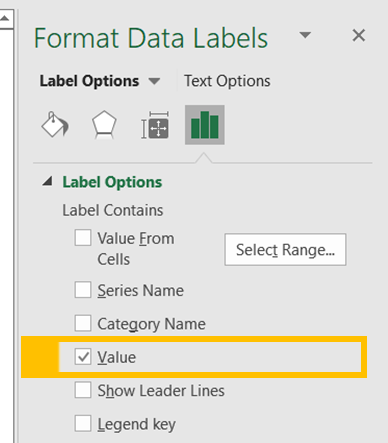
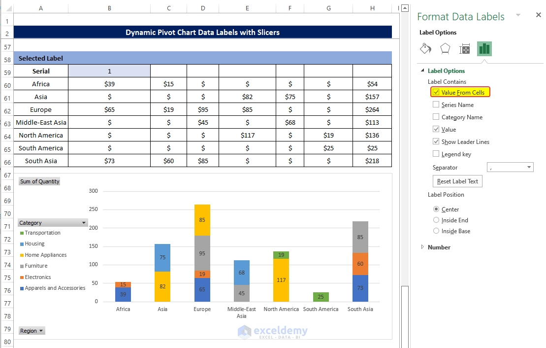
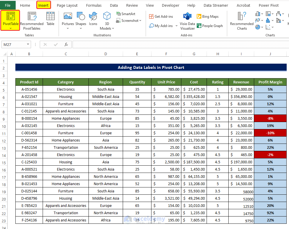
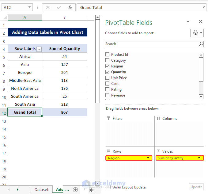
Add data labels to pivot chart. Formal ALL data labels in a pivot chart at once I go through the post, as per the article: Change the format of data labels in a chart, you may select only one data labels to format it. However, you may change the location of the data labels all at once, as you can see in screenshot below: I would suggest you vote for or leave your comments in the thread: Format Data Labels (Ex: Alignment ... › documents › excelHow to change/edit Pivot Chart's data source/axis/legends in ... If you want to change the data source of a Pivot Chart in Excel, you have to break the link between this Pivot Chart and its source data of Pivot Table, and then add a data source for it. And you can do as follows: Step 1: Select the Pivot Chart you will change its data source, and cut it with pressing the Ctrl + X keys simultaneously. How to Customize Your Excel Pivot Chart Data Labels Check the box that corresponds to the bit of pivot table or Excel table information that you want to use as the label. For example, if you want to label data markers with a pivot table chart using data series names, select the Series Name check box. If you want to label data markers with a category name, select the Category Name check box. Data Labels in Excel Pivot Chart (Detailed Analysis) Then add a Pivot Chart from the PivotTable Analyze tab. Next, you will notice that there is a data label option, but we want to add it manually from a range of cells. Click on the Plus sign right next to the Chart, then from the Data labels, click on the More Options. After that, in the Format Data Labels, click on the Value From Cells.
chandoo.org › wp › change-data-labels-in-chartsHow to Change Excel Chart Data Labels to Custom Values? May 05, 2010 · First add data labels to the chart (Layout Ribbon > Data Labels) Define the new data label values in a bunch of cells, like this: Now, click on any data label. This will select “all” data labels. Now click once again. At this point excel will select only one data label. How to Add Data to a Pivot Table: 11 Steps (with Pictures) - wikiHow Go to the spreadsheet page that contains your data. Click the tab that contains your data (e.g., Sheet 2) at the bottom of the Excel window. 3 Add or change your data. Enter the data that you want to add to your pivot table directly next to or below the current data. Add Value Label to Pivot Chart Displayed as Percentage I have created a pivot chart that "Shows Values As" % of Row Total. This chart displays items that are On-Time vs. items that are Late per month. The chart is a 100% stacked bar. I would like to add data labels for the actual value. Example: If the chart displays 25% late and 75% on-time, I would like to display the values behind those %'s ... chandoo.org › wp › budget-vs-actual-chart-free-templateFree Budget vs. Actual chart Excel Template - Download May 16, 2018 · Step 10: Add data labels to both lines. Select the lines one at a time (remember, the lines are invisible, so just click where they are supposed to be or use the format box to select them). Now use the + button to add data labels. In older versions of Excel, you need to use either ribbon or menus to add labels.
How do you add labels to a pivot table in Excel? How do I label rows in a pivot table? Right-click an item in the pivot field. In the Field Settings dialog box, click the Layout & Print tab. Add a check mark to Repeat item labels, then click OK. How do you customize a pivot table? How to make row labels on same line in pivot table? - ExtendOffice Click any cell in your pivot table, and the PivotTable Tools tab will be displayed. 2. Under the PivotTable Tools tab, click Design > Report Layout > Show in Tabular Form, see screenshot: 3. And now, the row labels in the pivot table have been placed side by side at once, see screenshot: w.sunybroome.edu › basic-computer-skills › functionsSpreadsheet Terminology - SUNY Broome Community College An Excel spreadsheet contains 256 columns that are labeled with the letters of the alphabet. When the column labels reach letter "Z" they continue on with AA, AB, AC..... AZ and then BA, BB, BC.....BZ etc. Column / Bar Chart: A column or bar chart is a style of chart that is used to summarize and compare categorical data. The length of each bar ... Create Dynamic Chart Data Labels with Slicers - Excel Campus You basically need to select a label series, then press the Value from Cells button in the Format Data Labels menu. Then select the range that contains the metrics for that series. Click to Enlarge Repeat this step for each series in the chart. If you are using Excel 2010 or earlier the chart will look like the following when you open the file.
how to add data labels into Excel graphs — storytelling with data
Add or remove data labels in a chart - support.microsoft.com Add data labels to a chart Click the data series or chart. To label one data point, after clicking the series, click that data point. In the upper right corner, next to the chart, click Add Chart Element > Data Labels. To change the location, click the arrow, and choose an option. If you want to ...
Dynamically Label Excel Chart Series Lines • My Online ...
peltiertech.com › copy-pivot-table-pivot-chartCopy a Pivot Table and Pivot Chart and Link to New Data Jul 15, 2010 · -the pivot chart, or the pivot table, or both, are moved into another sheet (the chart with cut-paste, pivot with the option-Move Pivot Table) This action, of moving the chart or pivot table will add an absolute path to the data source : ‘Book1 only pivot table.xlsx’!Table1
Pivot Chart Formatting Changes When Filtered - Peltier Tech
spreadsheeto.com › pivot-tablesHow to Create a Pivot Table in Excel - Spreadsheeto To add data columns into the table, drag and drop the desired field into ‘Column Labels’, ‘Row Labels’, or ‘Values’ (these 3 are also covered in more detail later). This example setup would list the data in rows separated by ‘Location’ and ‘Item’.

How to Customize Your Excel Pivot Chart Data Labels - dummies
Add a data label on Pivot Chart - social.technet.microsoft.com With .SeriesCollection (1).Points (i) .HasDataLabel = True. .DataLabel.Text = Worksheets ("Sheet2").Range ("a" & position_total).Value. position_total = position_total + 1. End With. End With. Next. End Sub. Select the Pivot chart, then run the macro "data_label".

Dynamically Label Excel Chart Series Lines • My Online ...
pandas - How to add data label value in bar chart in python pivot tabel ... How to add data label value in bar chart in python pivot tabel dataframe. import pandas as pd import numpy as np import matplotlib.pyplot as plt employees = {'Name of Employee': ['Jon','Mark','Tina','Maria','Bill','Jon','Mark','Tina','Maria','Bill','Jon','Mark','Tina','Maria','Bill','Jon','Mark','Tina','Maria','Bill'], 'Sales': [1000,300,400,500,800,1000,500,700,50,60,1000,900,750,200,300,1000,900,250,750,50], 'Quarter': [1,1,1,1,1,2,2,2,2,2,3,3,3,3,3,4,4,4,4,4], 'Country': ...

Excel charts: add title, customize chart axis, legend and ...
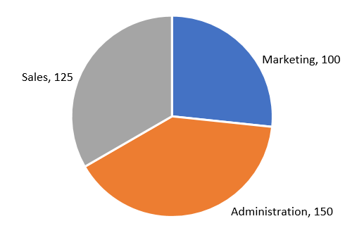
How do I add labels to my pivot chart? - Firstlawcomic Select the plot area of the pie chart. Right-click the chart. Select Add Data Labels. Select Add Data Labels. In this example, the sales for each cookie is added to the slices of the pie chart. How do you change the axis labels on a pivot chart? Right-click the category labels you want to change, and click Select Data. In the Horizontal (Category) Axis Labels box, click Edit.

Google Workspace Updates: Get more control over chart data ...
Include Grand Totals in Pivot Charts • My Online Training Hub Step 1: Load data to the Data Model. Insert a new PivotTable and at the dialog box check the 'add this data to the Data Model' box: Note: Excel 2010 users will need to load the data to Power Pivot via the Power Pivot tab > Add Linked Table. Then from the Power Pivot window Home tab > Insert PivotTable.

Custom Data Labels with Colors and Symbols in Excel Charts ...
How to update or add new data to an existing Pivot Table in Excel And here's the resulting Pivot Table: Change the Source Data for your Pivot Table. In order to change the source data for your Pivot Table, you can follow these steps: Add your new data to the existing data table. In our case, we'll simply paste the additional rows of data into the existing sales data table.

Bar charts with long category labels; Issue #428 November 27 ...
support.google.com › docs › answerAdd & edit a chart or graph - Computer - Google Docs Editors Help Double-click the chart you want to change. At the right, click Customize. Click Gridlines. Optional: If your chart has horizontal and vertical gridlines, next to "Apply to," choose the gridlines you want to change. Make changes to the gridlines. Tips: To hide gridlines but keep axis labels, use the same color for the gridlines and chart background.

How to Add Data Labels to your Excel Chart in Excel 2013
Adding Data Labels to a Pivot Chart with VBA Macro ActiveSheet.ChartObjects ("Cluster Overview").Activate ActiveChart.FullSeriesCollection (1).DataLabels.Select For i = 1 To Range ("PivotTable1 [Project '#]").Count ActiveChart.FullSeriesCollection (1).Points (i).DataLabel.Select Selection.Formula = Range ("PivotTable1 [Project '#]").Cells (i, 1) Next i Any help you can give will be great.
How to Show Percentages in Stacked Column Chart in Excel ...
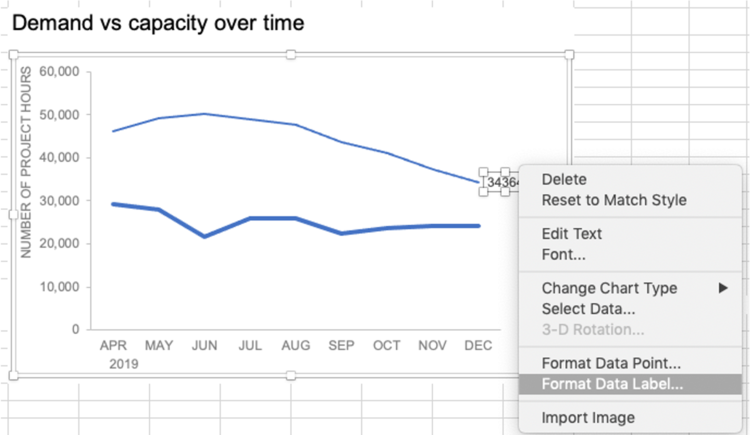
Change the format of data labels in a chart To get there, after adding your data labels, select the data label to format, and then click Chart Elements > Data Labels > More Options. To go to the appropriate area, click one of the four icons ( Fill & Line, Effects, Size & Properties ( Layout & Properties in Outlook or Word), or Label Options) shown here.
Data Labels in Excel Pivot Chart (Detailed Analysis) - ExcelDemy

Custom data labels in a chart

Directly Labeling Your Line Graphs | Depict Data Studio

Custom data labels in a chart

How to insert data labels to a Pie chart in Excel 2013

How to add live total labels to graphs and charts in Excel ...

Excel charts: add title, customize chart axis, legend and ...

Apply Custom Data Labels to Charted Points - Peltier Tech

How to Customize Your Excel Pivot Chart Data Labels - dummies

Adding rich data labels to charts in Excel 2013 | Microsoft ...
/simplexct/BlogPic-idc97.png)
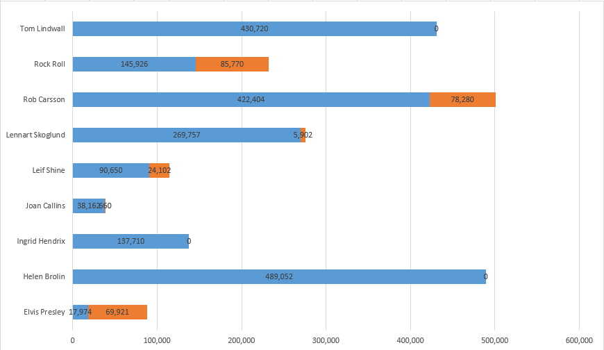
How to Create a Bar Chart With Labels Inside Bars in Excel

Add Total Values for Stacked Column and Stacked Bar Charts in ...

Dynamic Number Format for Millions and Thousands - PK: An ...

How to add or move data labels in Excel chart?
How to Create a Pareto Chart in Excel – Automate Excel

How to Add Axis Labels to a Chart in Excel | CustomGuide

How to make a pie chart in Excel
Data Labels in Excel Pivot Chart (Detailed Analysis) - ExcelDemy

Excel: Clustered Column Chart with Percent of Month ...

Color Negative Chart Data Labels in Red with downward arrow
Data Labels in Excel Pivot Chart (Detailed Analysis) - ExcelDemy
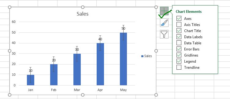
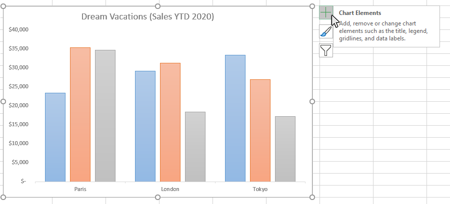
How to Add and Remove Chart Elements in Excel
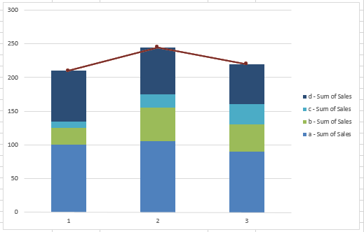
How-to Add a Grand Total Line on an Excel Stacked Column ...
How to fix wrapped data labels in a pie chart | Sage Intelligence

Adding rich data labels to charts in Excel 2013 | Microsoft ...

Add Total Values for Stacked Column and Stacked Bar Charts in ...
how to add data labels into Excel graphs — storytelling with data
Adding data labels in stacked chart Excel Nprintin... - Qlik ...
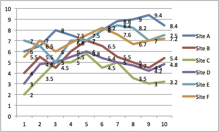
Directly Labeling Excel Charts - PolicyViz

Creating Pie Chart and Adding/Formatting Data Labels (Excel)
Move and Align Chart Titles, Labels, Legends with the Arrow ...
Change the look of chart text and labels in Numbers on Mac ...
How to Add Data Tables to a Chart in Excel - Business ...
Post a Comment for "44 add data labels to pivot chart"